Abstraction in the function concept

A century ago mathematics witnessed a dramatic enlargement and abstraction of this central concept. Let's explore some of the mind-expanding new possibilities...

Please enjoy this free extended excerpt from Lectures on the Philosophy of Mathematics, published with MIT Press 2021, an introduction to the philosophy of mathematics with an approach often grounded in mathematics and motivated organically by mathematical inquiry and practice. This book was used as the basis of my lecture series on the philosophy of mathematics at Oxford University.

Lectures on the Philosophy of Mathematics, MIT Press 2021

Abstraction in the function concept

The increasing rigor in mathematical analysis was also a time of increasing abstraction in the function concept. What is a function? In the naive account, one specifies a function by providing a rule or formula for how to compute the output value y in terms of the input value x. We all know many examples, such as y = x² + x + 1 or y = e^x or y = sin x. But do you notice that already these latter two functions are not expressible directly in terms of the algebraic field operations? Rather, they are transcendental functions, already a step up in abstraction for the function concept.

The development of proper tools for dealing with power series led mathematicians to consider other more general function representations, such as power series and Fourier series, as given here for the exponential function e^x and the sawtooth function s(x):

\( e^x = \sum_{n = 0}^\infty\frac{x^n}{n!}\qquad\qquad s(x) = \frac{2}{π}\sum_{n = 0}^\infty \frac{(-1)^{n + 1}}{n}\sin(nx). \)

The more general function concept provided by these kinds of representations enabled mathematicians to solve mathematical problems that were previously troubling. One can look for a solution of a differential equation, for example, by assuming that it will have a certain series form and then solve for the particular coefficients, ultimately finding that indeed the assumption was correct and there is a solution of that form. Fourier used his Fourier series to find solutions of the heat equation, for example, and these series are now pervasive in science and engineering.

The Devil's staircase

Let us explore a few examples that might tend to stretch one's function concept. Consider the Devil's staircase, pictured below.

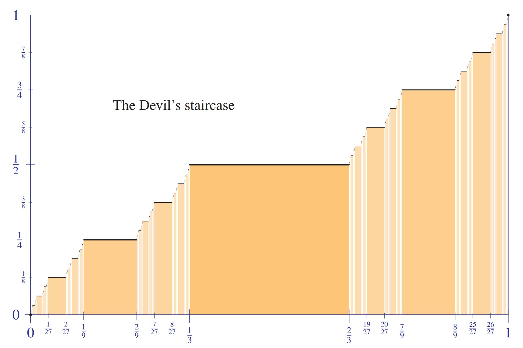
This function was defined by Cantor using his middle-thirds set, now known as the Cantor set, and serves as a counterexample to what might have been a certain natural extension of the fundamental theorem of calculus, since it is a continuous function from the unit interval to itself, which has a zero derivative at almost every point with respect to the Lebesgue measure, yet it rises from 0 to 1 during the interval. This is how the Devil ascends from 0 to 1 while remaining almost always motionless.

To construct the function, one starts with value 0 at the left and 1 at the right of the unit interval. Interpolating between these, one places constant value 1/2 on the entire middle-third interval; this leaves two intervals remaining, one on each side. Next, one places interpolating values 1/4 and 3/4 on the middle-thirds of those intervals, and so on, continuing successively to subdivide. This defines the function on the union of all the resulting middle-thirds sections, indicated in orange in the figure, and because of the interpolation, the function continuously extends to the entire interval. Since the function is locally constant on each of the middle-thirds intervals, the derivative is zero there, and those intervals add up to full measure one. The set of points that remain after omitting all the middle-thirds intervals is the Cantor set.

Space-filling curves

Next, consider the phenomenon of space-filling curves. A curve is a continuous function from the one-dimensional unit interval into a space, such as the plane, a continuous function c:[0,1] → ℝ². We can easily draw many such curves and analyze their mathematical properties.

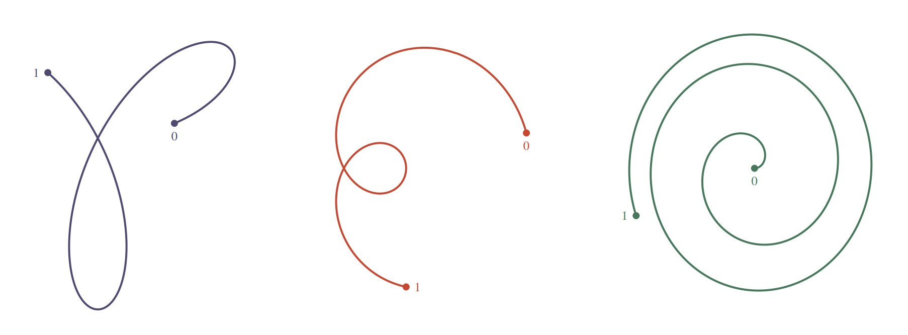
A curve in effect describes a way of traveling along a certain path: one is at position c(t) at time t. The curve therefore begins at the point c(0); it travels along the curve as time t progresses; and it terminates at the point c(1). Curves are allowed to change speed, cross themselves, and even to move backward on the same path, retracing their route. For this reason, one should not identify the curve with its image in the plane, but rather the curve is a way of tracing out that path.

Since the familiar curves that are easily drawn and grasped seem to exhibit an essentially one-dimensional character, it was a shocking discovery that there are space-filling curves, which are curves that completely fill a space. Peano produced such a space-filling curve, a continuous function from the unit interval to the unit square, with the property that every point in the square is visited at some time by the curve. Let us consider Hilbert's space-filling curve, shown here, which is a simplification.

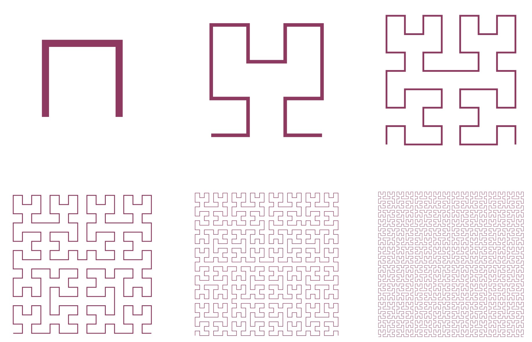
The Hilbert curve can be defined by a limit process. One starts with a crude approximation, a curve consisting of three line segments, as in the figure at the upper left; each approximation is then successively replaced by one with finer detail, and the final Hilbert curve itself is simply the limit of these approximations as they get finer and finer. The first six iterations of the process are shown here. Each approximation is a curve that starts at the lower left and then wriggles about, ultimately ending at the lower right. Each approximation curve consists of finitely many line segments, which we should imagine are traversed at uniform speed. What needs to be proved is that as the approximations get finer, the limiting values converge, thereby defining the limit curve.

One can begin to see this in the approximations to the Hilbert curve above. If we travel along each approximation at constant speed, then the halfway point always occurs just as the path crosses the center vertical line, crossing a little bridge from west to east (look for this bridge in each of the six iterations of the figure — can you find it?). Thus, the halfway point of the final limit curve h is the limit of these bridges, and one can see that they are converging to the very center of the square. So h(1/2) = (1/2, 1/2). Because the wriggling is increasingly local, the limit curve will be continuous; and because the wriggling gets finer and finer and ultimately enters every region of the square, it follows that every point in the square will occur on the limit path. So the Hilbert curve is a space-filling curve. To my way of thinking, this example begins to stretch, or even break, our naive intuitions about what a curve is or what a function (or even a continuous function) can be.

Conway base-13 function

Let us look at another such example, which might further stretch our intuitions about the function concept. The Conway base 13 function C(x) is defined for every real number x by inspecting the tridecimal (base 13) representation of x and determining whether it encodes a certain secret number, the Conway value of x. Specifically, we represent x in tridecimal notation, using the usual ten digits 0,...,9, plus three extra numerals ⊕, ⊖, and ⊙, having values 10, 11 and 12, respectively, in the tridecimal system. If it should happen that the tridecimal representation of x has a final segment of the form

\( ⊕a_0a_1\cdots a_k⊙b_0b_1b_2b_3\cdots, \)

where the a_i and b_j use only the digits 0 through 9, then the Conway value C(x) is simply the number

\(a_0a_1\cdots a_k.b_0b_1b_2b_3\ldots,\)

understood now in decimal notation. And if the tridecimal representation of x has a final segment of the form

\( { ⊖ }a_0a_1\cdots a_k{ ⊙ }b_0b_1b_2b_3\cdots,\)

where again the a_i and b_j use only the digits 0 through 9, then the Conway value C(x) is the number

\(- a_0a_1\cdots a_k.b_0b_1b_2b_3\ldots,\)

in effect taking ⊕ or ⊖ as a sign indicator for C(x). Finally, if the tridecimal representation of x does not have a final segment of one of those forms, for example, if it uses the ⊕ numeral infinitely many times or if it does not use the ⊙ numeral at all, then we assign the default value C(x) = 0.

Some examples may help illustrate the idea:

\(\begin{eqnarray*} x\qquad\qquad\qquad\qquad & ↦ &\quad C(x)\\ 12.35432{ ⊕ }3{ ⊙ }14159265\cdots & ↦ & \quad 3.14159265\cdots\\ 1.231{ ⊖ }2{ ⊙ }718281828\cdots & ↦ &\quad \llap{-}2.718281828\cdots\\ -1342{ ⊖ }{ ⊕ }12{ ⊕ }52.123{ ⊙ }7686767\cdots & ↦ &\quad52123.7686767\cdots\\ 1.2{ ⊕ }3{ ⊖ }4{ ⊕ }5{ ⊖ }6{ ⊕ }7{ ⊖ }8{ ⊕ }\cdots & ↦ &\quad 0 \end{eqnarray*} \)

The point is that we can easily read off the decimal value of C(x) from the tridecimal representation of x. On the left, we have the input number x, given in tridecimal representation, and on the right is the encoded Conway value C(x), in decimal form, with a default value of 0 when no number is encoded. Note that we ignore the tridecimal point of x in the decoding process.

Let us look a little more closely at the Conway function to discover its fascinating features. The key thing to notice is that every real number y is the Conway value of some real number x, and furthermore, you can encode y into the final segment of x after having already specified an arbitrary finite initial segment of the tridecimal representation of x. If you want the tridecimal representation of x to start in a certain way, go ahead and do that, and then simply add the numeral ⊕ or ⊖ after this, depending on whether y is positive or negative, and then list off the decimal digits of y to complete the representation of x, using the numeral ⊙ to indicate where the decimal point of y should be. It follows that C(x) = y. Because we can specify the initial digits of x arbitrarily, before the encoding of y, it follows that every interval in the real numbers, no matter how tiny, will have a real number x, with C(x) = y. In other words, the restriction of the Conway function to any tiny interval results in a function that is still onto the entire set of real numbers.

Consequently, if we were to make a graph of the Conway function, it would look totally unlike the graphs of other, more ordinary functions. Here is my suggestive attempt to represent the graph:

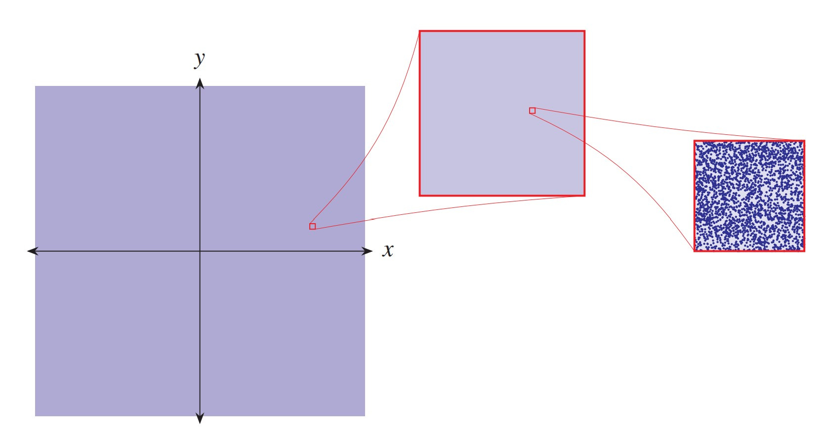
The values of the function are plotted in blue, you see, but since these dots appear so densely in the plane, we cannot easily distinguish the individual points, and the graph appears as a blue mass. When I draw the graph on a chalkboard, I simply lay the chalk sideways and fill the board with dust.

But the Conway function is indeed a function, with every vertical line having exactly one point, and one should imagine the graph as consisting of individual points ( x, C(x) ). If we were to zoom in on the graph, as suggested in the figure, we might hope to begin to discern these points individually. But actually, one should take the figure as merely suggestive, since after any finite amount of magnification, the graph would of course remain dense, with no empty regions at all, and so those empty spaces between the dots in the magnified image are not accurate. Ultimately, we cannot seem to draw the graph accurately in any fully satisfactory manner.

Another subtle point is that the default value of 0 actually occurs quite a lot in the Conway function, since the set of real numbers x that fail to encode a Conway value has full Lebesgue measure. In this precise sense, almost every real number is in the default case of the Conway function, and so the Conway function is almost always zero. We could perhaps have represented this aspect of the function in the graph with a somewhat denser hue of blue lying on the x-axis, since in the sense of the Lebesgue measure, most of the function lies on that axis. Meanwhile, the truly interesting part of the function occurs on a set of measure zero, the real numbers x that do encode a Conway value.

Notice that the Conway function, though highly discontinuous, nevertheless satisfies the conclusion of the intermediate value theorem: for any a < b, every y between f(a) and f(b) is realized as f(c) for some c between a and b.

We have seen three examples of functions that tend to stretch the classical conception of what a function can be. Mathematicians ultimately landed with a very general function concept, abandoning all requirements functions must be defined by a formula of some kind; rather, a function is simply a certain kind of relation between input and output: a function is any relation for which an input gives at most one output, and always the same output.

In some mathematical subjects, the function concept has evolved further, growing horns in a sense. Namely, for many mathematicians, particularly in those subjects using category theory, a function f is not determined merely by specifying its domain X, and the function values f(x) for each point in that domain x ∈ X. Rather, one must also specify what is called the codomain of the function, the space Y of intended target values for the function f : X → Y. The codomain is not the same as the range of the function, because not every y ∈ Y needs to be realized as a value f(x). On this concept of the function, the squaring function s(x) = x² on the real numbers can be considered as a function from ℝ to ℝ or as a function from ℝ to [0,∞), and the point would be that these would count as two different functions, which happen to have the same domain ℝ and the same value x² at every point x in that domain; but because the codomains differ, they are different functions. Such a concern with the codomain is central to the category-theoretic conception of morphisms, where with the composition of functions f ∘ g, for example, one wants the codomain of g to align with the domain of f.

Subscribe now for fresh weekly content on the mathematics and philosophy of the infinite.

Or, to support my work, you can buy me a coffee.

Continue reading more about this topic in the book:

Lectures on the Philosophy of Mathematics, MIT Press 2021